What's the problem?
The Parabolic Constant Mystery

Where is the Parabola?
The Parabolic Constant Mystery

Manas Shetty, Prajwal DSouza, Sparsha Kumari, Vinton Adrian Rebello

This work began with a familiar 3Blue1Brown feeling: a constant shows up where it has no obvious business being. In particular, pi appearing in unexpected contexts made us wonder whether other constants have similar geometric fingerprints. The case that caught our attention was a connection between parabolas and squares.

We spent about eight months trying different ways to understand it. Most attempts were clumsy. Eventually a much cleaner picture appeared: an average-distance problem in a square can be turned into the length of a parabolic arc.

After sitting on the idea for nearly three years, we are finally sharing it for SOME3.

This was made with viewX, a small visualization library used for the mathematical animations on this website. It is still in development and still a little buggy. :)

We also owe a lot to Matt Parker's video "There is only One True Parabola" (Stand-up Maths). The idea that all parabolas are similar is the key reason a constant can appear here at all.

Start with a unit square. Pick a point Q at random on its boundary. What is the average distance from Q to the square's center C?

By average distance, we mean: take all the possible distances, add them, and divide by how many distances were counted. For a continuous boundary, that idea becomes a limiting process.

The answer is approximately 0.5738967... This number is P/4, where P is the Universal Parabolic Constant. Its value is about 2.295587149... That raises the question: our problem is about a square, so where is the parabola?

It could be a coincidence. But when π appears in a strange place, we usually go looking for a circle. 3B1B has a whole video built on that instinct. Here we do the same thing with P: look for the hidden parabola.

What do you think is the average distance between any two points inside a unit square? Take a guess. :D

Move the slider to choose your answer. The points A and B above are draggable. :)

Check
Continue

It is about 0.52140. More precisely, it is

$$\color{#e3a0cd}{8\left(0.0416{\color{#ffffff}{P}}-0.030473\right)}$$
and exactly it is

$$\color{#e3a0cd}{8\left(\frac{\color{#ffffff}{P}}{24}-\frac{\sqrt{2}}{30}+\frac{1}{60}\right)}$$

Strange combination of numbers, but there is a P in it. :)
There are more examples like this, mostly involving a unit square.

Center-Point Distance
Corner-Perimeter Distance

Center-Point Distance
Corner-Perimeter Distance

Here is a related problem.
What do you think is the average distance between the center and any point 'inside' the unit square?

Take a guess. :D

Point B above is draggable. :)

Check
Continue

It is about 0.38259785. Exactly, it is

\(\color{#e3a0cd}{\frac{\color{#ffffff}{P}}{6}}\)

Yep. There's a P here too.

Now leave the square for a moment. A problem about a Shrinking Random Walk appeared in Tom Yuster's April 2017 Math Horizons piece (pp. 32-33).

Consider a walker in a plane who starts at the origin and moves only east or north. At each step, he randomly chooses one of those directions. The step lengths shrink: the first step is √2, the second step is √2/2, the third step is √2/4, and so on.

There are infinitely many steps, but you can choose how many to show. :)

After infinitely many steps, how far do you expect the walker to be from the starting point, the origin?
Call that distance D.

The question is: what is the average value of D?

How could we calculate it?
This looks far from the square problem, but it has the same central object: an average. (That is not the path length √2 + √2/2 + ...; it is the distance from the origin to the endpoint.)

We can start by simulating the walk for about 30 steps and recording where it ends. The later steps are tiny, so after a few steps the endpoint is already close to its final position. From there, we compute the distance D from the origin and repeat the experiment a few times.

Add another trial

After looking at these values, what do you think is the average value?


Check
Continue

The answer is 2.295587149... Yes: it is P. It appears here too.
This problem has no visible square, but it still asks for an average.

So why does the same constant appear? What does this have to do with the parabola?
Here is the hint: the endpoint of the walk is not as shapeless as it first looks. Run many trials and mark the final positions, where the walker lands after infinitely many steps.

More trials? Move the slider. :)

Does it look familiar now?

So, what is the Universal Parabolic Constant?

Start with something familiar: what is pi?
For any circle, take half of its circumference and divide by the radius. The answer is always the same constant: π. Something similar happens for parabolas.

Circle

\(π = \frac{\text{Enclosing Arc}}{Radius}\)


= 2.2123
Parabola

\(P = \frac{\text{Enclosing Arc}}{Radius}\)


= 3.1545

Radius


In fact, the universal parabolic constant 2.295587... is an irrational number and is equal to \(√2 + ln(1+√2)\).
If we know the radius of a circle, we can compute its circumference. If we know the analogous "radius" of a parabola, we can compute the enclosing arc length.

Enclosing Arc = Universal Parabolic Constant x Radius

Wherever the same parabolic shape appears, the same ratio appears with it.

That is the point of the constant: it captures what stays unchanged when the shape is scaled. A circle can be drawn as a coin or a planet's orbit; the ratio stays π. A parabola can be small, wide, narrow, or scaled up; the corresponding ratio stays P.

Why do these constants appear?

Can we make more constants like this? Are they special to circles and parabolas? For a square of side length \(L\), the ratio of perimeter \(4L\) to diagonal \(\sqrt{2}L\) is always \(\frac{4}{\sqrt{2}}\).
Any family of similar shapes can produce ratios like this. All circles are similar, so π is constant across circles. The useful surprise is that all parabolas are similar too. See Matt's video (Stand-up Maths) for more details.

When we scale a shape, matching lengths scale together. Double a circle and both the radius and circumference double, so their ratio stays the same. The square's perimeter-to-diagonal ratio works the same way.

But what do radius and center even mean for a parabola?
First, what is a parabola?
One way to construct it is this: take a fixed point F and a fixed line L. Then collect every point Q whose distance from F equals its perpendicular distance from L.
That set of points is a parabola.

Move the slider to see more points that obey the same distance rule.

Before defining the parabolic constant, we need a few names.
The fixed point is the focus, usually denoted F. The vertex of the parabola, call it C, is the point closest to the fixed line L. Let that shortest distance be a. Now draw a line M through the focus F, parallel to L. It cuts the parabola at two points.

The two points are G and H drawn below.

Next

The point H, at horizontal distance 2a from the vertex C, will matter later.
The line FH is half the latus rectum of the parabola. We will use it as the parabola's analogue of a radius.
The full latus rectum, GH, plays the role of a diameter and has length 4a.

Keep these lengths in mind: HB has length a and CB has length 2a.
For example, if HB has length 0.5 units, then CB is 1 unit.

The arc GCH is the enclosed arc of the parabola, and FH is the radius-like length. The Universal Parabolic Constant P is the ratio between them:

Arc \(\color{#a585ff}{GCH}\color{#737373} = \color{#ffffff}P\color{#737373} \times \color{#ff7a7a}FH\)

Since GCH has length P times 2a, half of it, CH, has length P times a. So: $$Arc \; \color{#a585ff}{CH}\color{#737373} = \color{#ffffff}P\color{#737373} \times \color{#e3a0cd}a$$ Substituting the value of P gives: $$Arc \; \color{#a585ff}{CH}\color{#737373} = \color{#ffffff}2.295587..\color{#737373} \times \color{#e3a0cd}a$$

Here is one more property of the parabola. If you have seen basic calculus, this will be familiar; otherwise the picture below gives the intuition.

Consider the equation of a line
\(\color{#737373}{y = \color{#ffffff}{m}\color{#61bdff}{x}}\)

Taking one of the simplest parabolas, we see that
\(\color{#737373}{y = x^2 = \color{#ffffff}{x}\color{#61bdff}{x}}\)

The slope of the curve increases as you move away from the origin along the x axis. To see it, draw the tangent line at a point of interest and watch that tangent get steeper as the x coordinate increases.

A parabola is a curve whose slope changes linearly with the x coordinate. Notice that the tangent at H makes a 45 degree angle with the x axis. In other words, the slope at H (x = 2a) is 1.

Value of the x-coordinate

If you want the calculus check for the slope at H, here it is.

The equation of this parabola is

$$y = \frac{x^2}{4a}$$

The points C and H here are at (0, 0) and (2a, a), respectively.

You can check this directly:
1. \(y = 0 \) when \(x = 0 \) (the vertex C)
2. \(y = a \) when \(x = 2a \) (our point H)


Now, differentiate the equation of the parabola to get the slope at any point (x,y) on the parabola.
$$\frac{dy}{dx} = \frac{x}{2a}$$ At H, where x = 2a, \(dy/dx = 2a/2a\) = 1. So

At H, the tangent makes a 45 degree angle with the x axis.

Moving on.

A small detour. The Division of lines.

12/4 is 3. That's simple division.
Here is a physical version of division. I have a piece of ribbon of length 12. Can you turn it into a piece of ribbon of length 3?

I give you the big ribbon. You do something to it and give me back the small ribbon.

The direct method is straightforward:

1. Break the ribbon evenly into 4 pieces.
2. Keep one piece.

Next

That method works. But another version will be more useful for curves:

shrink the line segment by a factor of 4.

Next

This version transfers better to curves.

How do we divide a curve of length \( L \) and get a similar curve of length \( L/n \)?
Start with a line.


Scaling down both x and y by a factor of 4 gives the line segment we want. Its length is 3, which is 12/4.

We can do the same with any curve. Suppose a curve has length 20 and we want a similar curve whose length is divided by 4. We scale the whole curve instead of chopping off a piece.


Continue

Now we have a way to divide a curve while preserving its shape. We will use that in a moment.

What is average?

The original problem asks for an average value. So what exactly are we averaging?

For a finite set of cases, the average is simple: go through all possible cases, add them, and divide by the number of cases. For example, the average value (expected value) of a die roll is: $$\color{#a585ff}{A} \color{#737373}= \frac{\color{#e3a0cd}{1} \color{#4a76e5}+ \color{#e3a0cd}{2} \color{#4a76e5}+ \color{#e3a0cd}{3} \color{#4a76e5}+ \color{#e3a0cd}{4} \color{#4a76e5}+ \color{#e3a0cd}{5} \color{#4a76e5}+ \color{#e3a0cd}{6}}{\color{#ff7a7a}{6}} $$

If there are 9 people in the room, all with height 6 ft, what is the average height?

$$ \color{#a585ff}{A} \color{#737373}= \frac{ \color{#e3a0cd}6 \color{#4a76e5}+ \color{#e3a0cd}6 \color{#4a76e5}+ \color{#e3a0cd}6 \color{#4a76e5}+ \color{#e3a0cd}6 \color{#4a76e5}+ \color{#e3a0cd}6 \color{#4a76e5}+ \color{#e3a0cd}6 \color{#4a76e5}+ \color{#e3a0cd}6 \color{#4a76e5}+ \color{#e3a0cd}6 \color{#4a76e5}+ \color{#e3a0cd}6} {\color{#ff7a7a}{9}} $$

Here is a small trick that we will need later.

What is the average of the following numbers?
1, 6, 2, 2, 6, 2, 1, 1, 6

Rearrange them:

$$ \color{#a585ff}A \color{#737373}= \frac{\color{#ccc161}1 + 2 + 6 + \color{#adff7a}1 + 2 + 6 + \color{#ccc161}1 + 2 + 6}{\color{#ff7a7a}9} $$

Then the same average is simply: $$ \color{#a585ff}A \color{#737373}= \frac{ \color{#ccc161}1 + 2 + 6}{\color{#ff7a7a} 3} $$

Instead of averaging all 9 numbers, we can average 1, 2, 6 because the same block repeats.
If 10 people have an average height of 6 feet, adding 10 more people with the same average does not change the combined average.
Repeated symmetric pieces can be collapsed.

Average for 1, 2, 6, 1, 2, 6, 1, 2, 6
is the same as
Average for 1, 2, 6, 1, 2, 6, 1, 2, 6, 1, 2, 6, 1, 2, 6, 1, 2, 6, 1, 2, 6, 1, 2, 6, 1, 2, 6
is the same as
Average for 1, 2, 6


The square has the same kind of repetition. Instead of averaging over the whole boundary, we can use symmetry and focus on one side: what is the average distance between the center C and a point on the line AB?

Now we have a fixed point and a fixed line. That should sound suspiciously close to the definition of a parabola, but we still have not seen the curve.
It will appear after we rewrite the average geometrically.

The simpler problem

The reduced problem is this: a line of height 0.5 stands at a distance of 0.5 from point C. What is the average distance from C to a point on that line?

To make the arithmetic cleaner, scale the square by 2, so the distance CB is 1. The problem becomes: a line of height 1 stands at a distance of 1 from point C. What is the average distance from C to a point on that line?

In principle, we should sweep through every point on the line, add all the distances, and divide by the number of points. But a line has infinitely many points, so we need to approach the average by a limit.

Start with only a few sample points. For 2 points, use the endpoints A and B.

In this case, numerically the average for two lengths is

$$\color{#a585ff}A_{\color{#ff7a7a}2} \color{#737373}= \frac{ \color{#e3a0cd}CB \color{#737373}+ \color{#adff7a}CA}{\color{#ff7a7a} 2} $$

\( \color{#a585ff}A_{\color{#ff7a7a}2} \color{#737373}= \frac{ \color{#e3a0cd}1 \color{#737373}+ \color{#adff7a}\sqrt{2}}{\color{#ff7a7a} 2} \color{#737373}= \frac{ \color{#e3a0cd}1 \color{#737373}+ \color{#adff7a} 1.414..}{\color{#ff7a7a} 2} = \color{#ffffff} 1.207..\)

CA is square root of 2 by the Pythagorean theorem.

Now, how about 3? If we evenly divide the line into two, we can get three points. A, B and a midpoint E.

In this case, numerically the average for three lengths is

$$ \color{#a585ff}A_{\color{#ff7a7a}3} \color{#737373}= \frac{\color{#e3a0cd}CB \color{#737373}+ \color{#e7d9b6}CE \color{#737373}+ \color{#adff7a}CA}{\color{#ff7a7a} 3} $$

\( \color{#a585ff}A_{\color{#ff7a7a}3} \color{#737373}= \frac{ \color{#e3a0cd}1 \color{#737373}+ \color{#e7d9b6}\frac{\sqrt{5}}{2}\color{#737373}+ \color{#adff7a}\sqrt{2}}{\color{#ff7a7a} 3} \color{#737373}= \frac{ \color{#e3a0cd}1 \color{#737373}+ \color{#e7d9b6}1.118.. \color{#737373}+ \color{#adff7a} 1.414..}{\color{#ff7a7a} 3} = \color{#ffffff} 1.1773..\)

CE is square root of 5 divided by 2 by the Pythagorean theorem.

Our goal is the continuous average, so we need to understand \( \color{#a585ff}A_{\color{#ff7a7a}n} \) as \(n\) goes to infinity.

For 4 points, divide the line into 3 equal parts. For 5 points, divide it into 4 equal parts. For n points, divide it into \(n - 1\) equal parts.
Then average the distances from C to those sampled points.

Numerically, this works: add the sampled distances, divide by the number of samples, then let the number of samples grow.
But where is the parabola?

Can you see it?

The parabola is hidden in the averaging process.
Start with the roughest average: just 2 sample points. Remember this expression?

Add Scale down

$$ \color{#a585ff}A_{\color{#ff7a7a}2} \color{#737373}= \frac{ \color{#e3a0cd}CB \color{#737373}+ \color{#adff7a}CA}{\color{#ff7a7a} 2} = \frac{1 \color{#ffffff}+\color{#737373} \sqrt{2}}{2} $$

To average, add and then divide.

The first step is to add the lengths from each case. How do we add CA and CB as lengths?
Lay them end to end. The combined green and pink segment represents the sum.
Drag the slider to move the segment.

\( \color{#a585ff}A_{\color{#ff7a7a}2} \color{#737373}= \frac{ \color{#e3a0cd}CB \color{#737373}+ \color{#adff7a}CA}{\color{#ff7a7a} 2}\color{#737373} = \color{#ffffff}\frac{\color{#737373}1 + \sqrt{2}}{\color{#737373}2} \)

The next step is division. How do we divide a line without changing its shape?
We shrink it along both axes. Drag the slider to scale down along both x and y axes.

The length of the scaled-down segment \( \frac{ \color{#e3a0cd}CB}{\color{#ff7a7a} 2} \color{#737373}+ \frac{\color{#adff7a}CA}{\color{#ff7a7a} 2} \)
represents the sum \( \color{#a585ff}A_{\color{#ff7a7a}2} \)

Its length is the average distance for those 2 points.

Continue
Continue

Two sample points are too crude. Try 3.

Add Scale down

\( \color{#a585ff}A_{\color{#ff7a7a}3} \color{#737373}= \frac{ \color{#e3a0cd}CB \color{#737373}+ \color{#ffbe8f}CQ \color{#737373}+ \color{#adff7a}CA}{\color{#ff7a7a} 3} = \frac{1 \color{#ffffff}+ \color{#737373} \frac{\sqrt{5}}{2} \color{#ffffff}+\color{#737373} \sqrt{2}}{3} \)

Same idea: add, then divide.

First add the lengths from each case: CA, CQ, and CB. As before, lay CA, CQ, and CB end to end. The combined green line + orange line + pink line represents the sum.
Drag the slider to move the segments.

\( \color{#a585ff}A_{\color{#ff7a7a}3} \color{#737373}= \frac{ \color{#e3a0cd}CB \color{#737373}+ \color{#ffbe8f}CQ \color{#737373}+ \color{#adff7a}CA}{\color{#ff7a7a} 3} = \color{#ffffff} \frac{\color{#737373}1 + \frac{\sqrt{5}}{2} +\color{#737373} \sqrt{2} \color{#ffffff}}{\color{#737373} 3} \)

Now divide by 3.
Shrink the curve along both axes by a factor of 3. Drag the slider to scale down along both x and y axes.

The length of the scaled-down curve \( \frac{ \color{#e3a0cd}CB}{\color{#ff7a7a} 3} \color{#737373}+ \frac{ \color{#ffbe8f}CQ}{\color{#ff7a7a} 3} \color{#737373}+ \frac{\color{#adff7a}CA}{\color{#ff7a7a} 3} \)
represents the sum \( \color{#a585ff}A_{\color{#ff7a7a}3} \)

Its length is the average distance for those 3 points.

Continue
Continue

This should start to look familiar. Also notice that the order can be reversed: scale each segment down first, then add the scaled pieces. Divide each segment by 3 and then add them together.

$$ \frac{ \color{#e3a0cd}CB \color{#737373}+ \color{#ffbe8f}CQ \color{#737373}+ \color{#adff7a}CA}{\color{#ff7a7a} 3} $$ $$ \frac{ \color{#e3a0cd}CB}{\color{#ff7a7a} 3} \color{#737373}+ \frac{ \color{#ffbe8f}CQ}{\color{#ff7a7a} 3} \color{#737373}+ \frac{\color{#adff7a}CA}{\color{#ff7a7a} 3} $$
Do it in that order now.
For 3 points: sample 3 points, break line AB into 2 pieces, take the distances to the 3 points, divide each distance by 3, and add the pieces together.

For 4 points:
break line AB into 3 pieces, take the distances to the 4 points, divide each distance by 4, and add the pieces together.

Scale down Add

\( \color{#a585ff}A_{\color{#ff7a7a}4} \color{#737373}= \frac{ \color{#e3a0cd}CB}{\color{#ff7a7a} 4} \color{#737373}+ \frac{ \color{#ffbe8f}CQ}{\color{#ff7a7a} 4} \color{#737373}+ \frac{ \color{#ffbe8f}CK}{\color{#ff7a7a} 4} \color{#737373}+ \frac{\color{#adff7a}CA}{\color{#ff7a7a} 4} = \frac{1 \color{#ffffff}+ \color{#737373} \frac{\sqrt{10}}{3} \color{#ffffff}+ \color{#737373} \frac{\sqrt{13}}{3} \color{#ffffff}+\color{#737373} \sqrt{2}}{4} \)

Here we first divide each line segment by 4 and then add.

\( \color{#a585ff}A_{\color{#ff7a7a}4} \color{#737373}= \color{#ffffff} \frac{\color{#737373}1 \color{#ffffff}}{\color{#737373} 4} \color{#737373}+ \color{#ffffff} \frac{\color{#737373} \frac{\sqrt{10}}{3} \color{#ffffff}}{\color{#737373} 4} \color{#737373}+ \color{#ffffff} \frac{\color{#737373} \frac{\sqrt{13}}{3} \color{#ffffff}}{\color{#737373} 4} \color{#737373}+ \color{#ffffff} \frac{\color{#737373} \sqrt{2} \color{#ffffff}}{\color{#737373} 4} \)

Continue

Now add the scaled-down segments CA/4, CK/4, CQ/4, and CB/4.

As before, lay CA, CK, CQ, and CB end to end. The combined green line + orange lines + pink line represents the sum.
Drag the slider to move the segments.


The final curve made by the scaled segments represents our sum \( \color{#a585ff}A_{\color{#ff7a7a}4} \). The shape is getting harder to ignore.

Continue

Now the pattern is visible.
The algorithm for 4 points was:
Sample: 4 points, by breaking the line into 3 pieces.
Divide: divide each segment by 4.
Add: lay the 4 scaled segments end to end.


For n points: Sample: n points, by breaking the line into n - 1 pieces.
Divide: divide each segment by n.
Add: lay the n scaled segments end to end.

Scale down Add

\( \color{#a585ff}A_{\color{#ff7a7a}n} \color{#737373}= \frac{ \color{#e3a0cd}CB}{\color{#ff7a7a} n} \color{#737373}+ \frac{ \color{#ffbe8f}CQ_1}{\color{#ff7a7a} n} \color{#737373}+ ... \color{#737373}+ \frac{\color{#adff7a}CA}{\color{#ff7a7a} n} = \frac{1 \color{#ffffff}+ ... +\color{#737373} \sqrt{2}}{n} \)
\( \color{#a585ff}A_{\color{#ff7a7a}n} \color{#737373} = \frac{ \color{#e3a0cd}CB}{\color{#ff7a7a} n} \color{#737373}+ \frac{ \color{#ffbe8f}CQ_1}{\color{#ff7a7a} n} \color{#737373}+ ... \color{#737373}+ \frac{\color{#adff7a}CA}{\color{#ff7a7a} n} \)

\(= \color{#737373} \frac{1 \color{#ffffff}+ ... +\color{#737373} \sqrt{2}}{n} \)


Here we first divide each line segment by n and then add them.

\( \color{#a585ff}A_{\color{#ff7a7a}n} \color{#737373}= \color{#ffffff} \frac{\color{#737373}1 \color{#ffffff}}{\color{#737373} n} \color{#737373}+ \color{#ffffff} \frac{\color{#737373} \sqrt{1 + {(\frac{1}{n})}^2} \color{#ffffff}}{\color{#737373} n} \color{#737373}+ \color{#ffffff} \frac{\color{#737373} \sqrt{1 + {(\frac{2}{n})}^2} \color{#ffffff}}{\color{#737373} n} \color{#737373}+ ...+ \color{#ffffff} \frac{\color{#737373} \sqrt{2} \color{#ffffff}}{\color{#737373} n} \)

$$ \color{#a585ff}A_{\color{#ff7a7a}n} \color{#737373} = $$ $$ \color{#ffffff} \frac{\color{#737373}1 \color{#ffffff}}{\color{#737373} n} \color{#737373}+ \color{#ffffff} \frac{\color{#737373} \sqrt{1 + {(\frac{1}{n})}^2} \color{#ffffff}}{\color{#737373} n} $$ $$ \color{#737373}+ \color{#ffffff} \frac{\color{#737373} \sqrt{1 + {(\frac{2}{n})}^2} \color{#ffffff}}{\color{#737373} n} \color{#737373}+ ...+ \color{#ffffff} \frac{\color{#737373} \sqrt{2} \color{#ffffff}}{\color{#737373} n} $$

Continue

Now add the scaled-down segments.

As before, lay CA, CQ2, CQ3, CQ4, ... and CB end to end. The resulting curve represents the sum.
Drag the slider to move the segments.
Notice that the final point always lands at the midpoint of line AB.


The final curve made by scaled segments represents our sum \( \color{#a585ff}A_{\color{#ff7a7a}n} \).

With many points, it begins to look like a parabola.

At infinitely many points, this should be a parabola.

Continue

It is a parabola.

Wait. Before using that, we should prove it.

How do we know that the curve is really a parabola?

If the final curve is a parabola, its points should obey an equation of the form

$$ y = \frac{x^2}{4a} $$ A point on this curve has the form: $$ \left(x, \frac{x^2}{4a}\right) $$

Our goal is to show that, as the number of sampled points gets large (\( n \to \infty \)), points on our constructed curve approach this form.

Start with 3 points, so n = 3. Each line segment (CQ1, CQ2, and CQ3) contributes a point to the curve after scaling.

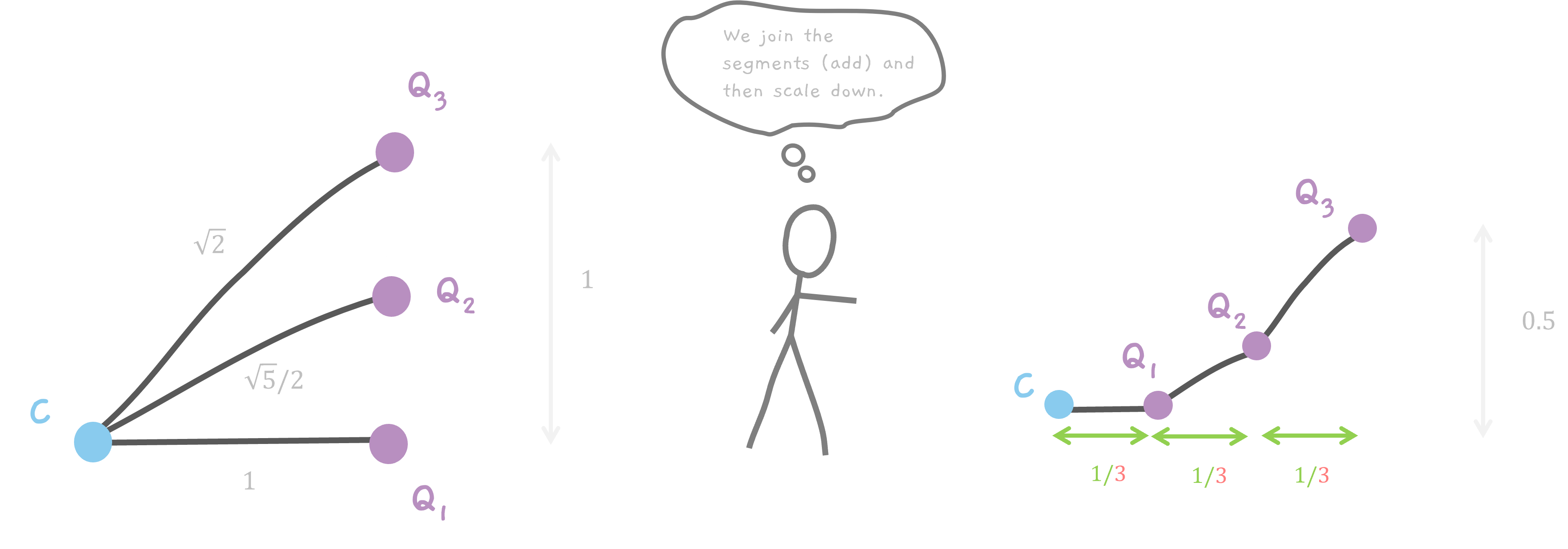
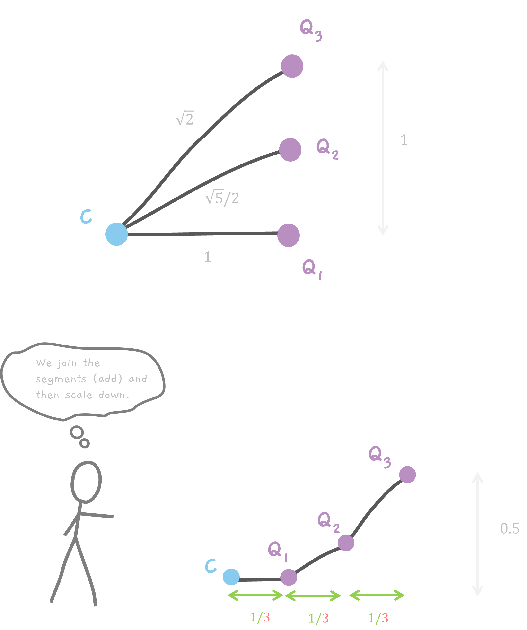
We want the final coordinates of Q1, Q2, and Q3. Take C as the origin.
There are two steps: add, then scale down. A point Q has different coordinates after each step.

Before adding the segments.
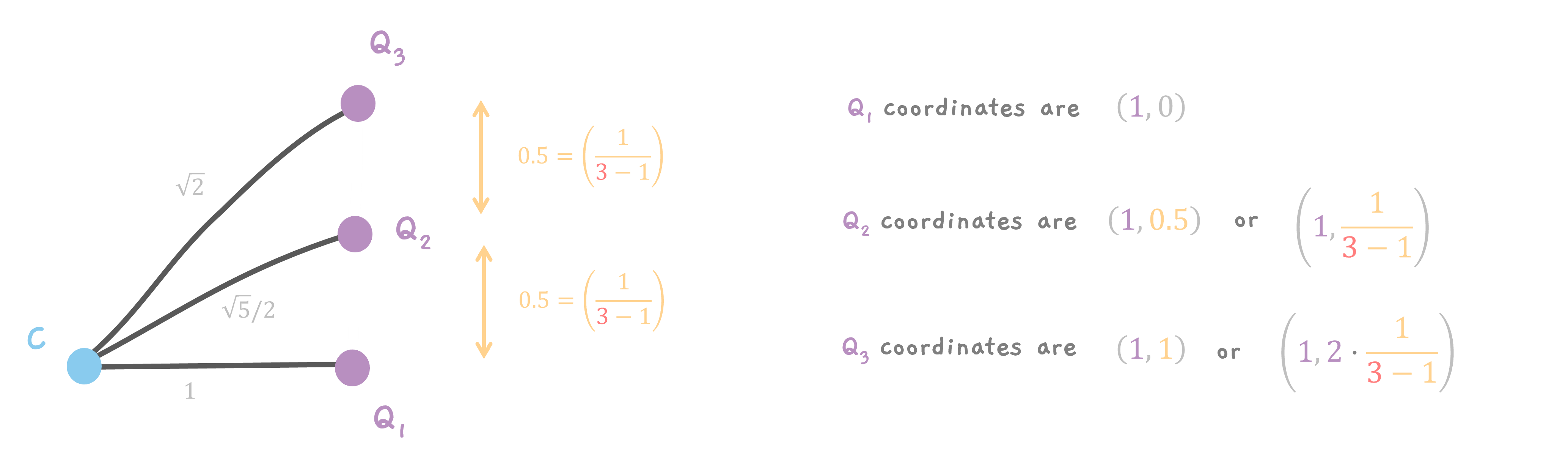
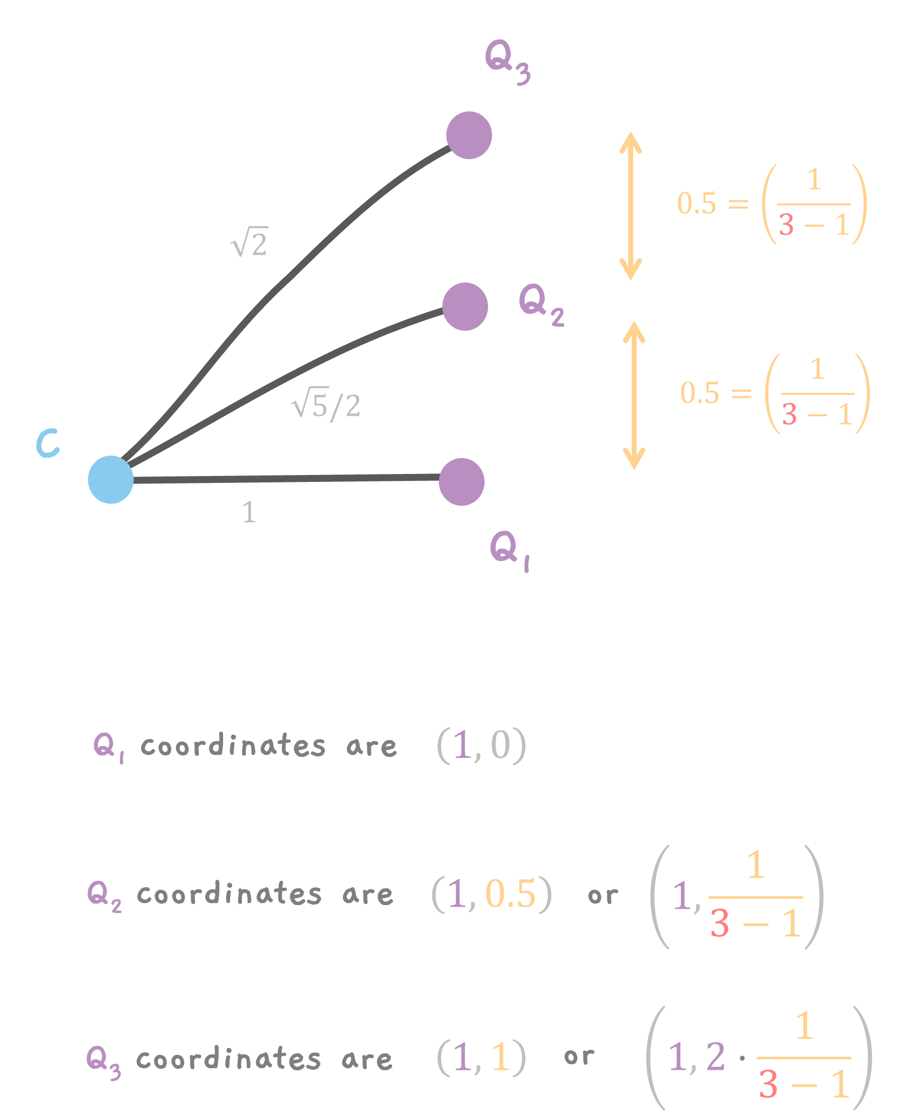
All the points are on line AB, so each x coordinate is 1. The y coordinate is a fraction of the length of AB. For n sample points, line AB is divided into n - 1 segments, so each segment has length 1/(n - 1). For 3 points, the distance between neighboring points is 1/(3 - 1), or 1/2.
So Q1 is at (1, 0), Q2 is at (1, 0.5), and Q3 is at (1, 1).

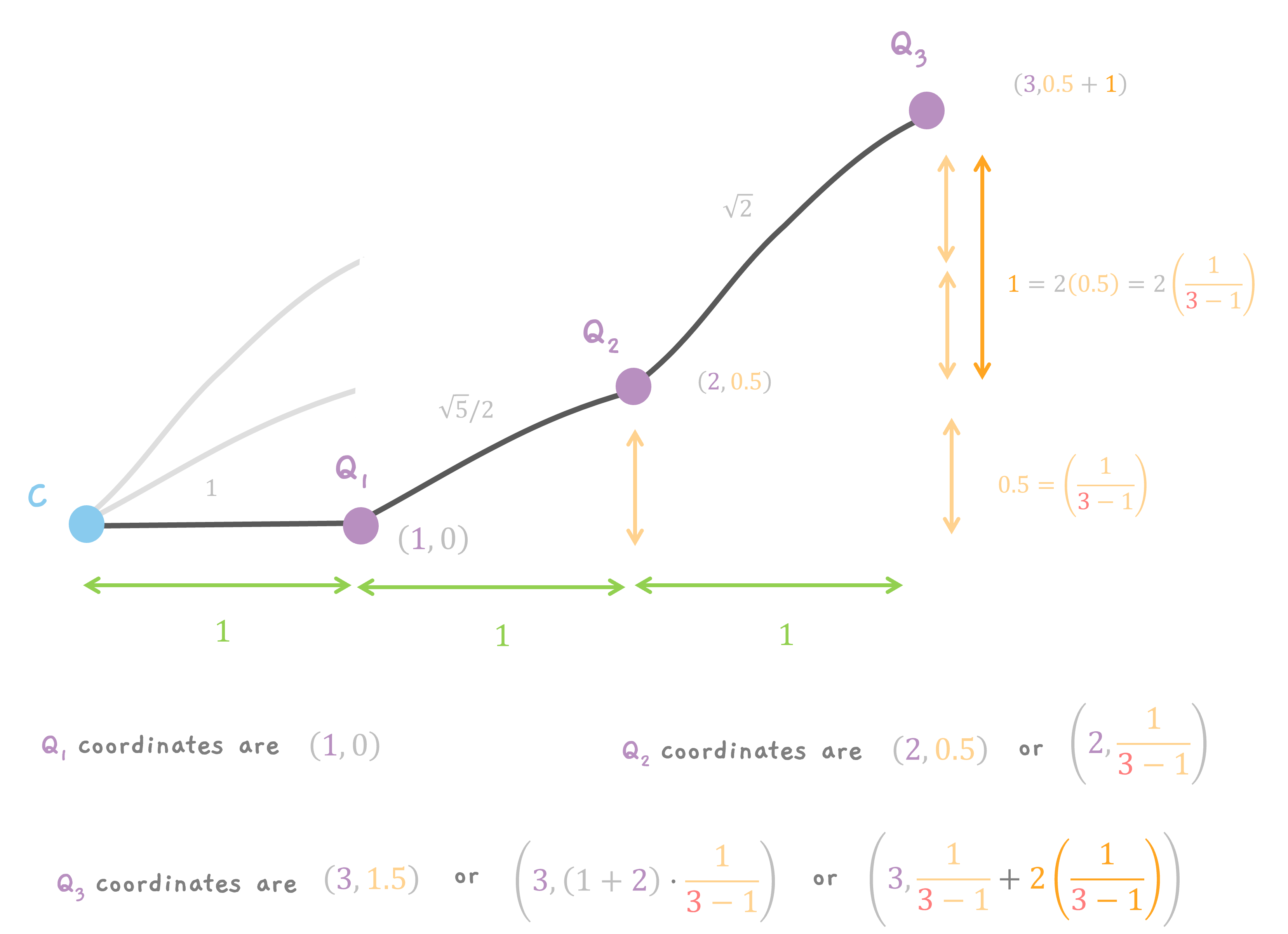
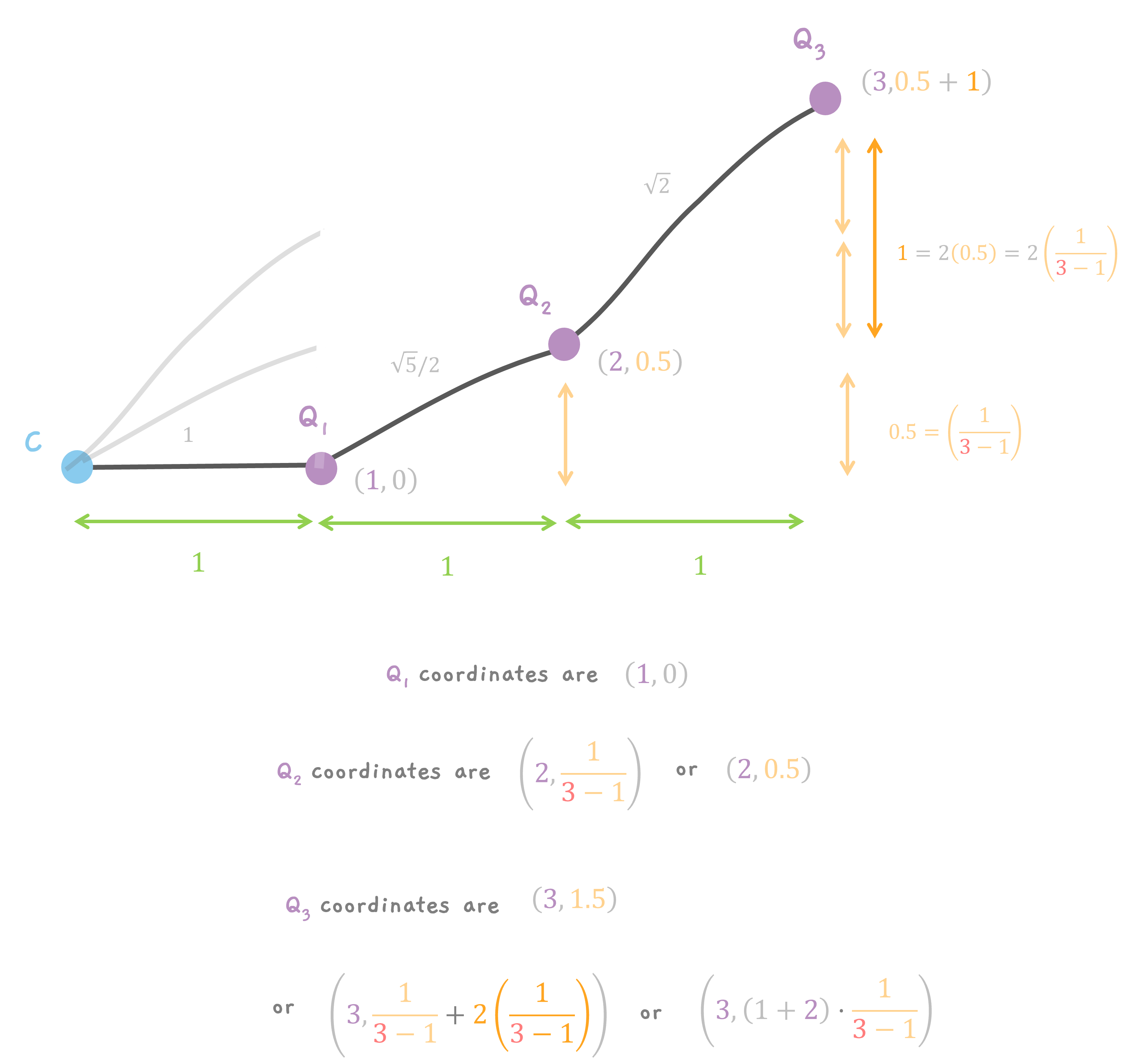
After adding the segments.
When the segments are laid end to end, the coordinates change. The x coordinates are easy: Q1 stays at x = 1, Q2 moves to x = 2, and Q3 moves to x = 3.
The y coordinates need one more step.
Q1 stays at y = 0. Q2 gets one half-step, so it moves to y = 0.5. Q3 gets two half-steps, giving 1, plus the earlier 0.5 from Q2. So its y coordinate becomes 0.5 + 1 = 1.5.
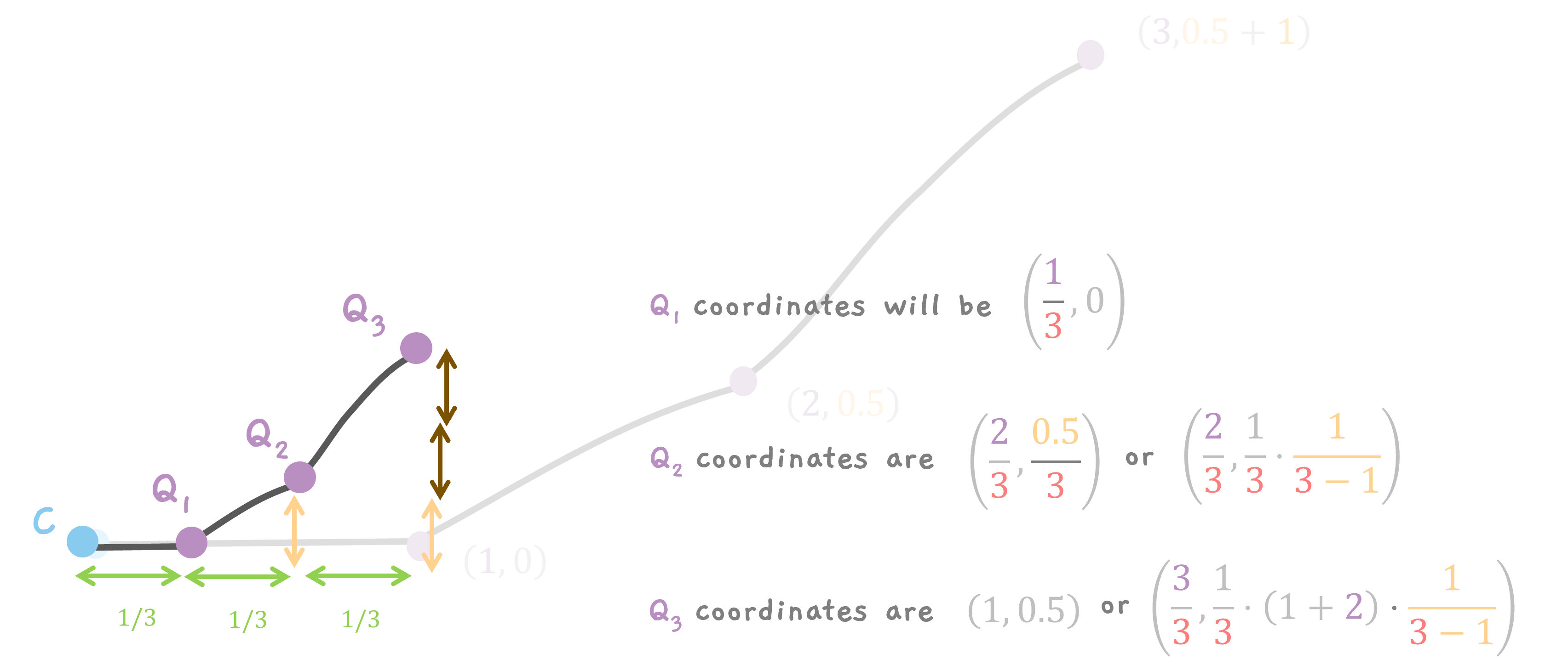
After scaling down.
Now scale the curve down by a factor of 3. The x coordinates are divided by 3: Q1 goes to x = 1/3, Q2 moves to x = 2/3, and Q3 moves to x = 3/3 = 1.
The y coordinates are divided by 3 too. Q1 stays at y = 0. Q2 goes from y = 0.5 to y = 0.5/3. Q3 goes from y = 1.5 to y = 1.5/3 = 0.5.
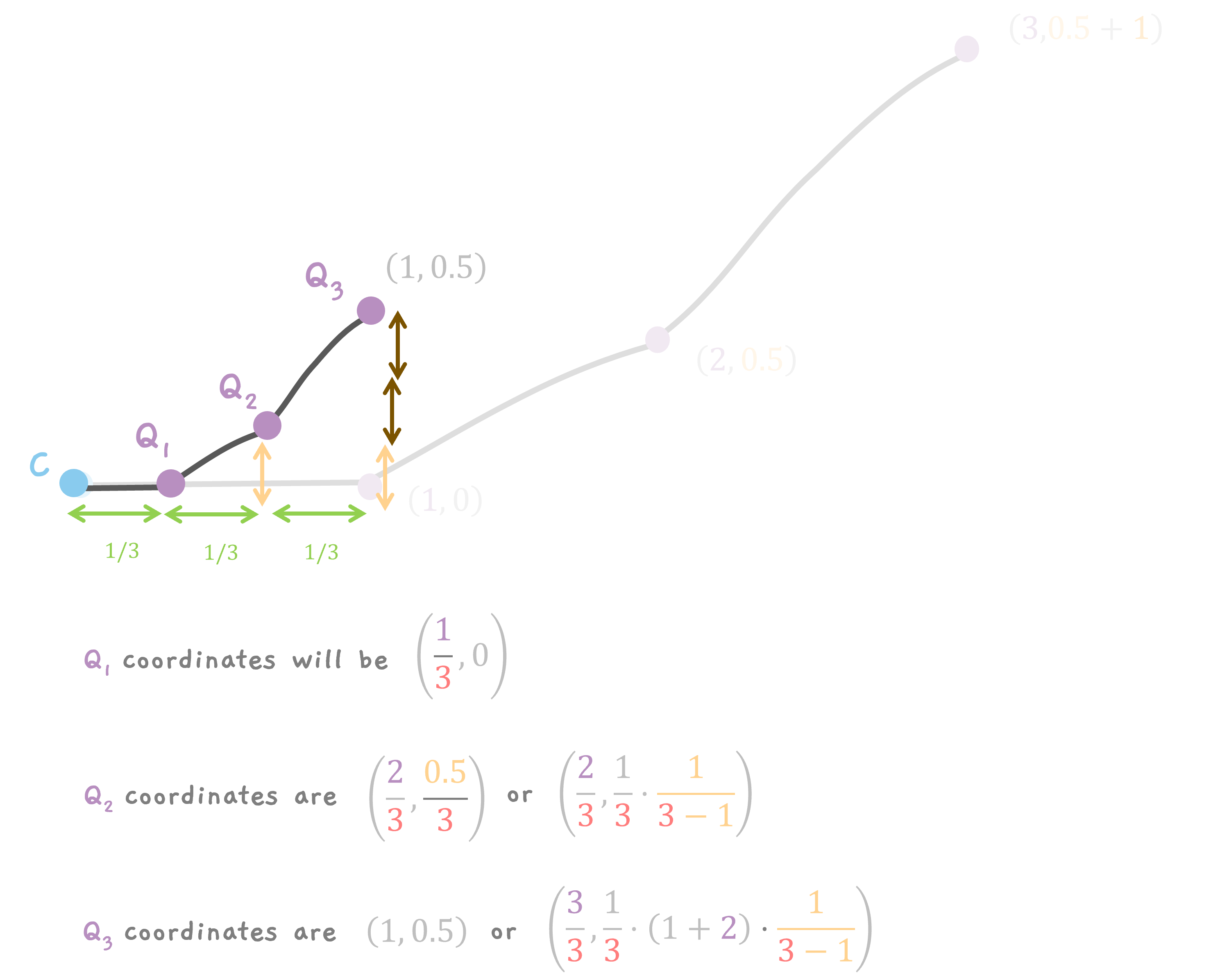
The coordinates now show the pattern.

Q1, the 1st point is at (1/3, 0).
Q2, the 2nd point is at (2/3, 0.5/3) or
$$ \left( \frac{2}{3}, \frac{1}{3}\cdot (1) \cdot \frac{1}{3 - 1} \right) $$ and Q3, the 3rd point is at (1, 0.5) or (3/3, 1.5/3) or
$$ \left( \frac{3}{3}, \frac{1}{3}\cdot (1 + 2) \cdot \frac{1}{3 - 1} \right) $$


For 4 sampled points, line AB is divided into 3 segments:

For n = 4, Q1, the 1st point is at (1/4, 0).
Q2, the 2nd point is at (2/4, 0.33/4) or
$$ \left( \frac{2}{4}, \frac{1}{4}\cdot (1) \cdot \frac{1}{4 - 1} \right) $$
Q3, the 3rd point is at (3/4, 1/4) or
$$ \left( \frac{3}{4}, \frac{1}{4}\cdot (1 + 2) \cdot \frac{1}{4 - 1} \right) $$ and Q4, the 4th point (final point) is at (1, 0.5) or (4/4, 2/4) or
$$ \left( \frac{4}{4}, \frac{1}{4}\cdot (1 + 2 + 3) \cdot \frac{1}{4 - 1} \right) $$

For this 4-point case in general,
the kth point Qk is at
$$ \left( \frac{k}{4}, \frac{1}{4}\cdot (1 + 2 + .. + (k - 1)) \cdot \frac{1}{4 - 1} \right) $$

The same pattern works for any n:
the kth point Qk is at
$$ \left( \frac{k}{n}, \frac{1}{n} \cdot (1 + 2 + .. + (k - 1)) \cdot \frac{1}{n - 1} \right) $$ Since the sum of the first \(k - 1\) integers is \((k - 1)k/2\), this becomes: $$ \left( \frac{k}{n}, \frac{1}{n} \cdot \left(\frac{(k - 1)k}{2}\right) \cdot \frac{1}{n - 1} \right) $$ After simplifying, when we sample n points, the kth point Qk is at
$$ \left( \frac{k}{n}, \frac{1}{2} \cdot \frac{k}{n} \cdot \frac{k - 1}{n - 1} \right) $$ This also explains why the final point always has y = 0.5. For the nth point: $$ \left( \frac{n}{n}, \frac{1}{2} \cdot \frac{n}{n} \cdot \frac{n - 1}{n - 1} \right) $$ which gives us: $$ \left( 1, 0.5 \right) $$

Now check what happens as the number of sampled points gets large (\( n \to \infty \)). Do the points approach the parabola equation?

As \( n \to \infty \), $$ \frac{k - 1}{n - 1} \thickapprox \frac{k}{n} $$ So, when \( n \to \infty \), the kth point is given by: $$ \left( \frac{k}{n}, \frac{1}{2} \cdot \frac{k}{n} \cdot \frac{k}{n} \right) $$ or $$ \left( \frac{k}{n}, \frac{1}{2} \cdot \left(\frac{k}{n}\right)^2 \right) $$ If we take x = k/n, then $$ \left(x, \frac{1}{2} \cdot \left(x\right)^2 \right) $$ or $$ \left(x, \frac{x^2}{4 \cdot 0.5} \right) $$ This is the equation we wanted. The limiting curve is a parabola.

This also gives us \( a = 0.5 \).

Since a = 0.5, H is at (2a, a), so the final point is H = (1, 0.5).

Before that, one loose end:

Why does the final point always land at the midpoint of AB?

X coordinate of the midpoint.
Look at the add-and-scale operation.

First, before scaling, each segment spans 1 unit in the x direction. So the unscaled curve spans n units in the x direction.
When it was 2 points, it spans 2 units in the x direction. When it was 3 points, it spans 3 units in the x direction. With n points, it spans n units in the x direction.

After scaling down by n, the x coordinate of the final point is 1, matching the x coordinate of line AB.

Y coordinate of the midpoint.
The y coordinate follows the same operation.

Before scaling, the curve spans different lengths in the y direction.
With 2 points, CB spans 0 units and CA spans 1 unit, for a total y span of 0 + 1.
After scaling down by 2, that becomes 0.5: the midpoint of line AB.

With 3 points, CB spans 0 units, CQ1 spans 1/2 units, and CA spans 1 unit, for a total y span of 0 + (1/2) + 1 = 1.5.
After scaling down by 3, that also becomes 0.5.

With n points, CB spans 0 units, CQ1 spans 1/(n - 1) units, CQ2 spans 2/(n - 1) units, and so on, with the final segment CA spanning 1 unit.

The total y span is therefore

\(S = 0 + \frac{1}{n - 1} + \frac{2}{n - 1} + \frac{3}{n - 1} + ... + \frac{n - 2}{n - 1} + \frac{n - 1}{n - 1} \)

\( = \frac{1}{n - 1}(1 + 2 + 3 + ... + (n - 2) + (n - 1)) \)

The sum of the natural numbers up to n - 1 is \(\frac{(n - 1)n}{2}\). Substituting that,

\(S = \frac{1}{n - 1}(\frac{(n - 1)(n)}{2}) \)

\(= (\frac{n}{2}) \)

So the unscaled curve spans n/2 in the y direction for n points. For 2 points, that is 2/2; for 3 points, it is 3/2, as we saw earlier.

After scaling down by n, n/2 becomes 1/2. The final point therefore has y coordinate 1/2, the midpoint of line AB.

We can also recognize the parabola geometrically.

The last segment , corresponding to the unscaled CA, always reaches the midpoint at a 45 degree angle. The segment slopes increase linearly. That is exactly the behavior we just saw for a parabola.
The midpoint on AB is our point H.


Remember the relationship from the parabola diagram:
if HB has length a, then CB has length 2a.
In our scaled square, CB is 1, so HB is 0.5.
That gives \(a = 0.5\).


Since the curve is a parabola and ends at the midpoint H of AB,
Remember?
Arc \(\color{#a585ff}{CH}\color{#737373} = \color{#ffffff}P\color{#737373} \times \color{#e3a0cd}a\)
The length of arc CH is P times a. Here a is the distance HB, which is 0.5.
Arc \(\color{#a585ff}{CH}\color{#737373} = \color{#ffffff}P\color{#737373} \times \color{#e3a0cd}0.5\)
So our calculated average is represented by

Arc \(\color{#a585ff}{CH}\color{#737373} = \frac{\color{#ffffff}P\color{#737373}}{\color{#e3a0cd}2}\)


Wait. That does not seem right.
We wanted \(P/4\) , not \(P/2\) .

The difference is the scale: we doubled the square to make the arithmetic cleaner. The original problem has side length 1.
For a square of side length 1, CB equals 1/2, so HB, or a, equals 1/4. For that square,
Arc \(\color{#a585ff}{CH}\color{#737373} = \color{#ffffff}P\color{#737373} \times \color{#e3a0cd}\frac{1}{4}\)

Arc \(\color{#a585ff}{CH}\color{#737373} = \frac{\color{#ffffff}P\color{#737373}}{\color{#e3a0cd}4}\)

which is the value we started with.


Now we can predict the average distance for any square.
For side length 1, it is P/4; for side length 2, it is P/2. In general, for a square with side length L, the average distance between its center and a point on its perimeter is

\(\color{#ffffff}\frac{P}{4}\color{#737373} \times \color{#e3a0cd}L\)


At the start, P/4 looked like a parabolic number dropped into a square problem. The square itself never draws a parabola. It only gives us a family of distances from the center to the boundary.

The parabola appears when we average those distances geometrically: use symmetry to keep one side of the square, lay the sampled lengths end to end, and shrink the result by the number of samples. As the samples get finer, that broken curve settles into a parabolic arc.

So P was doing exactly what P does: measuring a parabolic arc. In the unit square, that arc has a = 1/4, so its length is P/4. The square is how we sampled the distances. The averaging process is what drew the parabola.